I first made an RShiny app in graduate school when I first discovered it in a course I was taking. Simple, yet powerful applications. Of course, I used baseball data for fun outside of my assignments. The goal was to look at pitch data and break it down by location. I wanted to bring that back to make something with AAA data!
Recently, MiLB has been tracking pitch data using Statcast. I used 2024 data from the Salt Lake Bees (Angels AAA Affiliate) to make an RShiny app of pitch data. I don’t believe it is complete data, since not all stadiums have Statcast, but used what there was. I isolated on all swing, not including foul balls. My goal was to be able to allow a user to filter by hits, in-play, whiffs, pitcher, and date. The output would be pitch location, separated by pitch type, and associated events. In addition, I added a stacked bar chart for frequency of pitch types by events. Let’s see how it turned out!
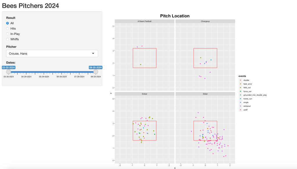
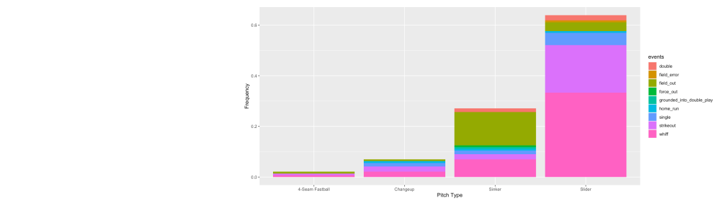
I didn’t do anything super fancy, but I think it is pretty neat. It is not BaseballSavant level but something you can do with open source data and software.
You can check it out here: http://cwatkins1123.shinyapps.io/Bees_Pitcher_App
Won’t gatekeeper code, so here it is for those interested:
bees <- read.csv("bees_pitch_data_24_data.csv")
bees$game_date <- as.Date(bees$game_date)
bees <- bees %>%
        mutate(events = ifelse(events == '', 'whiff', events))


tzone <- round(mean(bees$sz_top),2)
bzone <- round(mean(bees$sz_bot),2)
inKzone <- -.95
outKzone <- 0.95

kZone <- data.frame(
  x = c(inKzone, inKzone, outKzone, outKzone, inKzone)
  , y = c(bzone, tzone, tzone, bzone, bzone)
)


ui <- fluidPage(
  titlePanel("Bees Pitchers 2024", window ="Bees Pitchers 2024"),

  sidebarLayout(
    sidebarPanel(radioButtons("resultInput", "Result", choices = c("All", "Hits","In-Play","Whiffs"), selected = "All"),
                              uiOutput("playernameInput"),
                 sliderInput("dateInput",
                             "Dates:",
                             min = min(bees$game_date),
                             max = max(bees$game_date),
                             value = c(min(bees$game_date),max(bees$game_date)),
                             timeFormat="%m-%d-%Y")
    ),
    mainPanel(plotOutput("coolplot", width = "750px", height = "750px"),
              br(),
              plotOutput("coolplot2"),
              br(),
              textOutput("nrow"),
              br(),
              textOutput("credit"),
              br(),
              textOutput("signature"),
              br(),
              br())

  )
)
server <- function(input, output){
  output$playernameInput <- renderUI({
    selectInput("playernameInput", "Pitcher",
                choices = sort(unique(bees$player_name)),
                selected = "Crouse, Hans")
  })
  filtered <- reactive({
    if(is.null(input$resultInput)) {return(NULL)}
    else if(input$resultInput == "Hits"){
      bees %>%
        filter(player_name == input$playernameInput,
               events %in% c('single', 'double', 'triple', 'home_run'),
               game_date >= input$dateInput[1],
               game_date <= input$dateInput[2])
    }
    else if(input$resultInput == "In-Play"){
      bees %>%
        filter(player_name == input$playernameInput,
               description == "hit_into_play",
               game_date >= input$dateInput[1],
               game_date <= input$dateInput[2])
    }
    else if(input$resultInput == "Whiffs"){
      bees %>%
        filter(player_name == input$playernameInput,
               description %in% c("swinging_strike", "swinging_strike_blocked"),
               game_date >= input$dateInput[1],
               game_date <= input$dateInput[2])
    }
    else{
      bees %>%
        filter(player_name == input$playernameInput,
               game_date >= input$dateInput[1],
               game_date <= input$dateInput[2])
    }
  })

  output$coolplot <- renderPlot({
    if(is.null(input$playernameInput)) {return(NULL)}
    ggplot(filtered(), aes(x = plate_x, y = plate_z)) + geom_point(aes(col = events)) +
      scale_y_continuous(limits = c(0,5)) +
      scale_x_continuous(limits = c(-2.2, 2.2)) + coord_equal() +
      geom_path(aes(x, y), data = kZone, lwd = 1, col = "red", alpha = .5) +
      labs(x = "x", y = "z", title = "Pitch Location") +
      theme(plot.title = element_text(hjust = 0.5, face = "bold", size = 20),
            legend.title = element_text(face = "bold"))+facet_wrap(~pitch_name, ncol =2)
  }, height = 750, width = 750)

  output$coolplot2 <- renderPlot({
    if(is.null(input$playernameInput)) {return(NULL)}
    ggplot(filtered(),aes(fill = events, x = pitch_name))+
      geom_bar(aes(y = (..count..)/sum(..count..)))+
      labs(x = "Pitch Type", y = "Frequency")
  })


  output$nrow <- renderText({
    if(is.null(input$playernameInput)) {return(NULL)}
    nn <-nrow(filtered())
    paste("Based on your criteria, there were", nn, "pitches found.")
  })

  output$credit<- renderText({
    paste("Data pulled from BaseballSavant")
  })

  output$signature <- renderText({
    paste("By Chris Watkins, Ph.D.")
  })

}
shinyApp(ui = ui, server = server)