Everyone loves the whiff (also known as swinging strikes). Coaches, front offices, scouts, agents. Pitchers that don’t have good numbers on the surface but a high whiff % continue to get opportunities in MLB. Why? Well whiffs are an indicator of success for pitchers, especially relievers. If the bases are loaded with no outs, we’d want a strikeout rather than contact because a run can be scored on contact, even if it leads to an out. This will be a multipart series, starting with this one on the analytics and will go into modeling in subsequent parts. The goal is to find variables that influence whiffs and predict whiffs.
Finding the probability of a swing and miss can be done in a couple ways. We can be given that a hitter has swung or not. We will assume that the hitter has swung. For those probability lovers out there, assume event A is a swing and event B is a whiff. P(A and B) = P(A)P(B|A) from conditional probability. We will be focusing on P(B|A), the conditional probability that a hitter whiffed given they swung. Can argue back and forth about our assumption of a swing but the goal of this is not to determine what influences a swing, just that they whiff so I think this is the most logical way of going about it. Word of caution, there is some statistics here (exciting!) but do not fear I will break it down in simple terms!
Methodology
For this analysis I took data of every swing in 2021 from Baseball Savant. This was quite tedious because the limit for exporting data from Baseball Savant is 40,000 rows and the number of swing events was 334,881. So I meticulously took a couple weeks of data at a time resulting in 12 data sets and combined them together to get the full data set. I created a variable that is True when it was a whiff (swinging strike or swinging strike blocked) and False otherwise. Just as a glimpse into the issue data scientists must deal with, there were pitch types and pitch names that were empty like ” ”, which is different than an empty type which is NA/Null, so I had to fix that. I also made a variable for the ball-strike count and baseball state (i.e. 1 100 is 1 out runner on 1st). With this, the analysis can begin.
Results
We will slice and dice the data to look at whiff % in different aspects of the game. A simple group by for those data analyst out there. These are very simple but glean nice insights.
Let’s start simple with just the probability of a whiff (given a swing of course).
| Whiff % |
| 24% |
If a hitter swings, there is a 24% chance of a whiff.
We will now start to group by certain variables. First, by pitch name (without unknown pitch types).
| Pitch Name | Whiff % |
| Split-Finger | 36.2% |
| Slider | 33.9% |
| Knuckle Curve | 32.1% |
| Curveball | 30.9% |
| Changeup | 28.5% |
| Cutter | 22.0% |
| 4-Seam Fastball | 19.4% |
| Knuckleball | 14.7% |
| Sinker | 13.9% |
| Eephus | 11.5% |
| Fastball | 7.4% |
| Screwball | 0.0% |
Breaking it down by pitch we see a split-finger induces the most whiffs followed by a slider and knuckle curve. A couple things to note are that there was only 1 screwball recorded and fastball corresponds to 2-seam I believe. I asked about it, but haven’t heard back from Baseball Savant. However, the 2-seam fastball doesn’t show up anymore so I assume it is now just called fastball but maybe wrong on that.
Next, we will group by ball-strike count.
| Count | Whiff % |
| 0-2 | 27.2% |
| 0-1 | 26.5% |
| 1-2 | 25.6% |
| 0-0 | 25.1% |
| 1-0 | 24.5% |
| 1-1 | 24.5% |
| 2-1 | 22.1% |
| 2-2 | 22.1% |
| 2-0 | 21.7% |
| 3-1 | 18.6% |
| 3-2 | 18.0% |
| 3-0 | 16.0% |
To probably no one’s surprise, when being ahead of the count a pitcher will induce a whiff more often. What I find interesting is that 0-0 counts are 4th on this list which means that many times a pitcher won’t just throw a fastball down the middle for the first pitch. An indicator of a changing game.
Baseball state is up next. For those who are unfamiliar, there are 24 states a baseball game can be in during an inning. These are the combinations of outs and strikes. The first number will indicate the number of outs, and the the following 3 values will indicate runners on first, second, and third with a 1 indicating the base is occupied. For example, 1 010 would indicate 1 out and a runner on second base.
| State | Whiff % |
| 2 100 | 26.8% |
| 2 001 | 26.1% |
| 2 101 | 25.9% |
| 2 010 | 25.8% |
| 2 111 | 25.7% |
| 2 110 | 25.7% |
| 2 000 | 25.6% |
| 0 000 | 25.6% |
| 1 110 | 25.5% |
| 1 100 | 25.4% |
| 2 011 | 25.4% |
| 1 001 | 24.7% |
| 1 111 | 24.6% |
| 1 101 | 23.8% |
| 1 000 | 23.7% |
| 0 100 | 23.7% |
| 0 110 | 23.1% |
| 1 011 | 23.0% |
| 1 010 | 22.5% |
| 0 001 | 22.4% |
| 0 111 | 22.3% |
| 0 010 | 22.2% |
| 0 011 | 21.8% |
| 0 101 | 21.3% |
The top 5 states where whiffs were the highest were with two outs and runners on base. This isn’t entirely surprising as hitters are more aggressive to get runs in and pitchers are trying to avoid contact.
Finally, let’s explore both ball-strike count and baseball state together. I will spare you looking through 288 scenarios and just give you the top 10.
| State | Count | Whiff % |
| 0 110 | 3-0 | 44.4% |
| 0 100 | 3-0 | 40.0% |
| 1 010 | 3-0 | 33.3% |
| 2 100 | 0-2 | 32.8% |
| 0 100 | 0-2 | 32.3% |
| 0 000 | 0-2 | 32.1% |
| 0 000 | 2-0 | 32.1% |
| 2 100 | 0-1 | 31.5% |
| 1 001 | 2-0 | 31.3% |
| 0 000 | 0-0 | 30.7% |
Looking at the top 10 we see two trends. One is that on a 3-0 count and runners on hitters seem to be aggressive and whiff. Two, on an 0-2 count hitters must protect and pitchers don’t necessarily have to throw a strike.
We can go down a rabbit hole of grouping by more variables and get more and more specific. This will be the foundation for part 2 of this analysis which is sort of a naïve decision tree type model, but I will not spoil the surprise right now.
Let’s look at another important aspect, pitch location by pitch type.
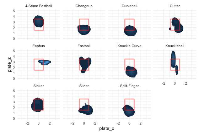
For this plot, the lighter the blue the more pitches in that area. This is from the catcher’s perspective. We can see clear trends that changeups and curveballs down as well as 4-seam fastballs up induce whiffs.
What else could influence a whiff? Let’s look at accelerations in the x direction (left/right, ax), and in the z direction (up/down) az.
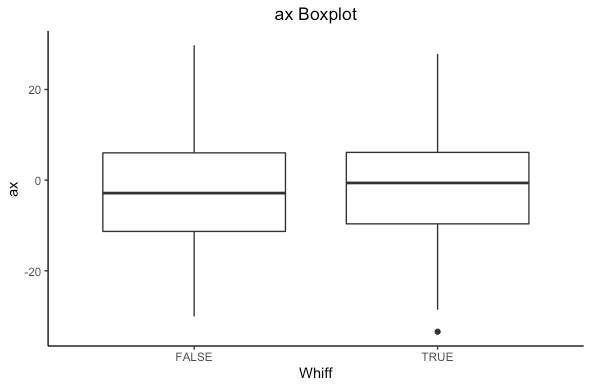
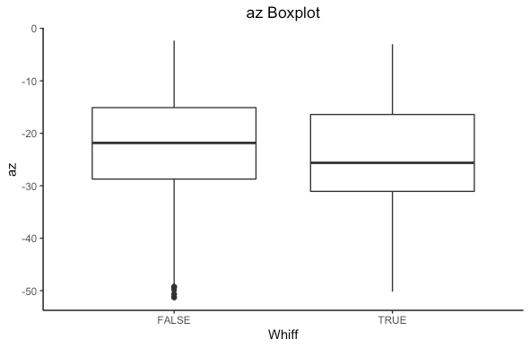
From the boxplot we see there is a different in medians for both plots. Statistically we can compute a t-test to see if there is a statistical difference in means. (For other R fans out there, I will be using t.test()). If we get a p-value less than 0.05 we have a statistically significant difference. If you are not well versed in statistics don’t worry, in simple terms it means the difference is actually a difference and not likely due to chance.
Welch Two Sample t-test
data:
swings[swings$swing_miss_tf == TRUE, "ax"] and swings[swings$swing_miss_tf == FALSE, "ax"]
t = 24.839, df = 143574, p-value < 2.2e-16
alternative hypothesis: true difference in means is not equal to 0
95 percent confidence interval:
0.9366943 1.0971813
sample estimates:
mean of x mean of y
-1.306053 -2.322991
Welch Two Sample t-test
data:
swings[swings$swing_miss_tf == TRUE, "az"] and swings[swings$swing_miss_tf == FALSE, "az"]
t = -57.324, df = 130076, p-value < 2.2e-16
alternative hypothesis: true difference in means is not equal to 0
95 percent confidence interval:
-2.166112 -2.022884
sample estimates:
mean of x mean of y
-24.67372 -22.57922 There is a statistical significance in both cases. In statistics language we can say that we reject the null hypothesis that there is no difference in means of ax and az based on if a hitter whiffs in favor of the alternative that there is a difference. Based on the confidence interval, we see that ax is higher when a hitter whiffs (positive is running right from the catchers perspective) and az is lower when a hitter whiffs (negative is dropping down). In simple terms, there is a difference that isn’t due to just chance.
Let’s repeat this for the spin rate of a 4-seam fastball and slider.
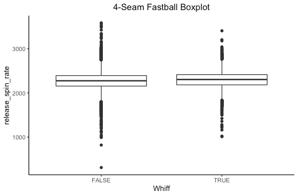
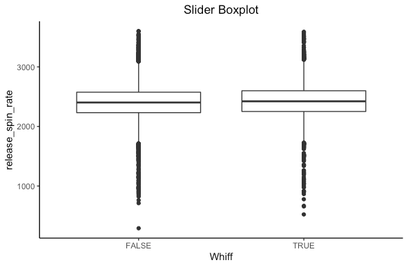
We see some sort of difference but not as clear here. What we need is more statistics!
Welch Two Sample t-test

data:
swings[swings$swing_miss_tf == TRUE & swings$pitch_name == "4-Seam Fastball", "release_spin_rate"] and swings[swings$swing_miss_tf == FALSE & swings$pitch_name == "4-Seam Fastball", "release_spin_rate"]
t = 19.642, df = 35360, p-value < 2.2e-16
alternative hypothesis: true difference in means is not equal to 0
95 percent confidence interval:
 23.38357 28.56781
sample estimates:
mean of x mean of y
 2297.987  2272.012
Welch Two Sample t-test
data:
swings[swings$swing_miss_tf == TRUE & swings$pitch_name == "Slider", "release_spin_rate"] and swings[swings$swing_miss_tf == FALSE & swings$pitch_name == "Slider", "release_spin_rate"]
t = 9.94, df = 43948, p-value < 2.2e-16
alternative hypothesis: true difference in means is not equal to 0
95 percent confidence interval:
17.44415 26.01333
sample estimates:
mean of x mean of y
2429.844 2408.115
Turns out there is a statistically significant difference in both cases. For the statistically inclined, we reject the null hypothesis that the mean spin rates are the same for 4-seam fastballs and sliders based on if a hitter whiffs in favor of the alternative that there is a difference. Based on the confidence intervals for both pitches, the spin rate is higher when a hitter whiffs. This makes sense, as higher spin rates have been shown to induce whiffs.
Conclusion
We see there are plenty of differences based on if a hitter whiffs. In this post we explored pitch type, pitch count, baseball state, baseball state + count, pitch location, accelerations, and spin rate. There certainly are more, and if I had unlimited time I could show more but also that would be an extremely long blog post. So I encourage you to explore more if you are interested! Now that we know there are differences, we can build models to predict a whiff. Next time I will be looking at a naïve model, which is inspired by Markov Chains (the probability of getting to the next state only depends on the current state) but is basically a decision tree.
