We saw in the previous post that there were quite a few differences when a hitter whiffs versus when they don’t. The data was sliced and diced in many ways like the count, state, and pitch. In this post I will be getting into some data science discussing a Naïve Model, which is basically just slicing and dicing the data and taking averages. For those data scientists out there it’s a very simple decision tree approach. The inspiration for this comes from a talk I saw at last year’s SABR Analytics conference where a Markov Chain approach was done. This inspired me to think that based on the variables we have we could find a probability that an event will happen. I used this approach to answer a question on a data questionnaire as part of the process for a baseball analytics position in baseball operations for the New York Mets. Unfortunately, did not get the position but was told the approach beat the other models submitted by a large margin. Got to the final round but a las, they went a different direction. I cannot say what that question was because of an NDA but will say that it was not the same as predicting whiffs, so I am not breaking any rules here.
Let’s get started!
Methodology
I will be using the exact same data set I used in the previous blog. However, I built one more variable called ‘platoon’ which is a value of True when there is a platoon advantage (i.e. Hitter and pitcher opposite handedness) and False otherwise.
The goal of this is to predict the probability of a whiff. Let’s get into a little data science. To do this I first split the data into a training and testing data set. Where 80% of the original data is in the training set and 20% is in the testing set. Alternatively, you could do 5-fold cross-validation [generally would do this but didn’t make as much sense here and going for simplicity]. The reason we split the data like this is because when a model is run for prediction it is on unseen data. Something to note is that the data is imbalanced, but not that bad. There is ~32% whiffs and the other ~68% is contact. Since we are predicting a probability rather than a true classification problem (Predicting a whiff or not. Either it happened or didn’t.) this is ok. One may argue it is fine for classification as well but that is an argument for another time. If you didn’t follow this, it is okay! Don’t necessarily need to know this. Time to slice and dice the training data set.
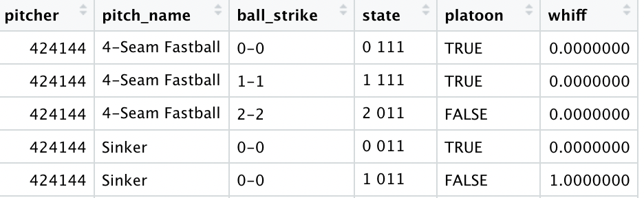
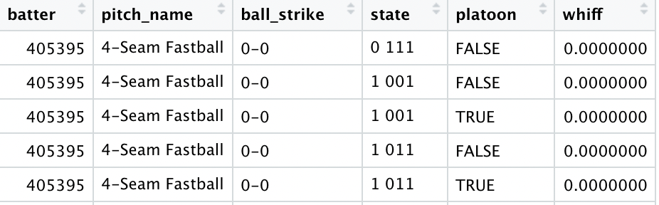
The first portion of this is the pitcher side where I will build a data set grouping by the pitcher, pitch name, count, baseball state, and platoon to get every combination. The second portion of this is the hitter side where it will be the same as previously mentioned but grouping by the hitter instead of the pitcher. Here is what they look like:
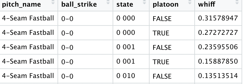
Then I grouped by pitch name, count, baseball state, and platoon. The reason for this is if a pitcher, hitter or both aren’t in the data sets built above this will break the model. Here is what it looks like.
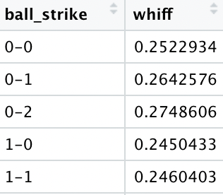
The last thing that I did was group by just count in case a pitch name, count, baseball state, and platoon combination was in the training set but not the test set.
Model
The model structure itself is simple at its core but could be confusing. If you find it too confusing feel free to jump ahead to results. Basically, we take the pitcher and hitter grouped data sets based on the pitcher and hitter respectively and find the corresponding probability and average them. If either the pitcher or batter don’t exist, we just use the one that does exist and data without pitcher or hitter. However, if both don’t exist, we will just use the grouped data without the pitcher and hitter. If the doesn’t exist, we take the data set just grouped by count. Confused? Let’s take an example.
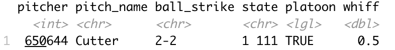
Say we have this scenario
| Pitcher | Hitter | Pitch Name | Count | State | Platoon |
| 650644 | 518735 | Cutter | 2-2 | 1 111 | True |
The batter data set doesn’t exist but the pitcher one does so we take that as one data point.
Then we take the data set without the pitcher or batter.
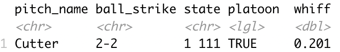
Then our final prediction is a (0.5+0.201)/2 = 0.3505 probability of a whiff.
Okay even I admit that is a lot. If you’ve made it this far, awesome! Let’s get into some results.
Results
I evaluated how well the model did with three metrics: MAE (Mean Absolute Error), accuracy (Over 50% probability is a predicted whiff), and AUC (Area Under Curve). For MAE, closer to a value of 0 is better and it measures how far on average the predictions were off by. Accuracy is the percentage of correct predictions assuming over a 50% probability is a predicted whiff. Finally, AUC (Area Under the Curve) measures how well a model fits the data with closer to 1 being better. I compared across several different model combinations and chose the best one.
Here are the results on predicting whiffs on the test set:
| MAE | Accuracy | AUC |
| 0.346 | 72.4% | 0.58 |
But what about class imbalance!? Yes there is some class imbalance, but this is why I calculate AUC.
Conclusion
I showed a simple at its core (yet confusing) decision tree model to predict a whiff, but is it good? The answer is yes, but why? Well, if we randomly simulated data from 0 to 1 and calculated metrics MAE would be 0.5 and accuracy 50%. So, this model performed about 44.5% better than chance in MAE and 22.4% better than chance in accuracy, and 16% better in AUC. There could very well be a better combination of variables out there that does better but what I find the most interesting is that sometimes the simple things are surprisingly good.
